Thresholding
Binary Decisions
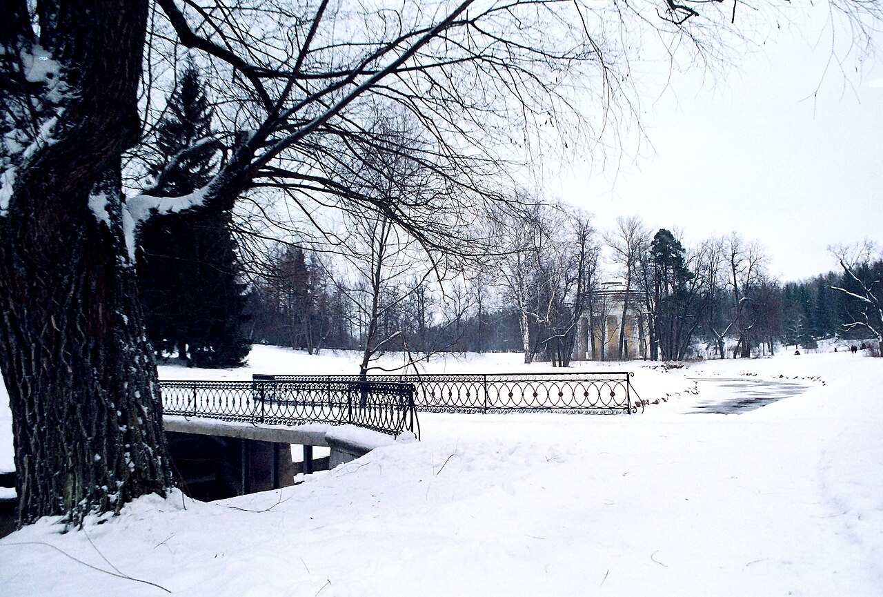
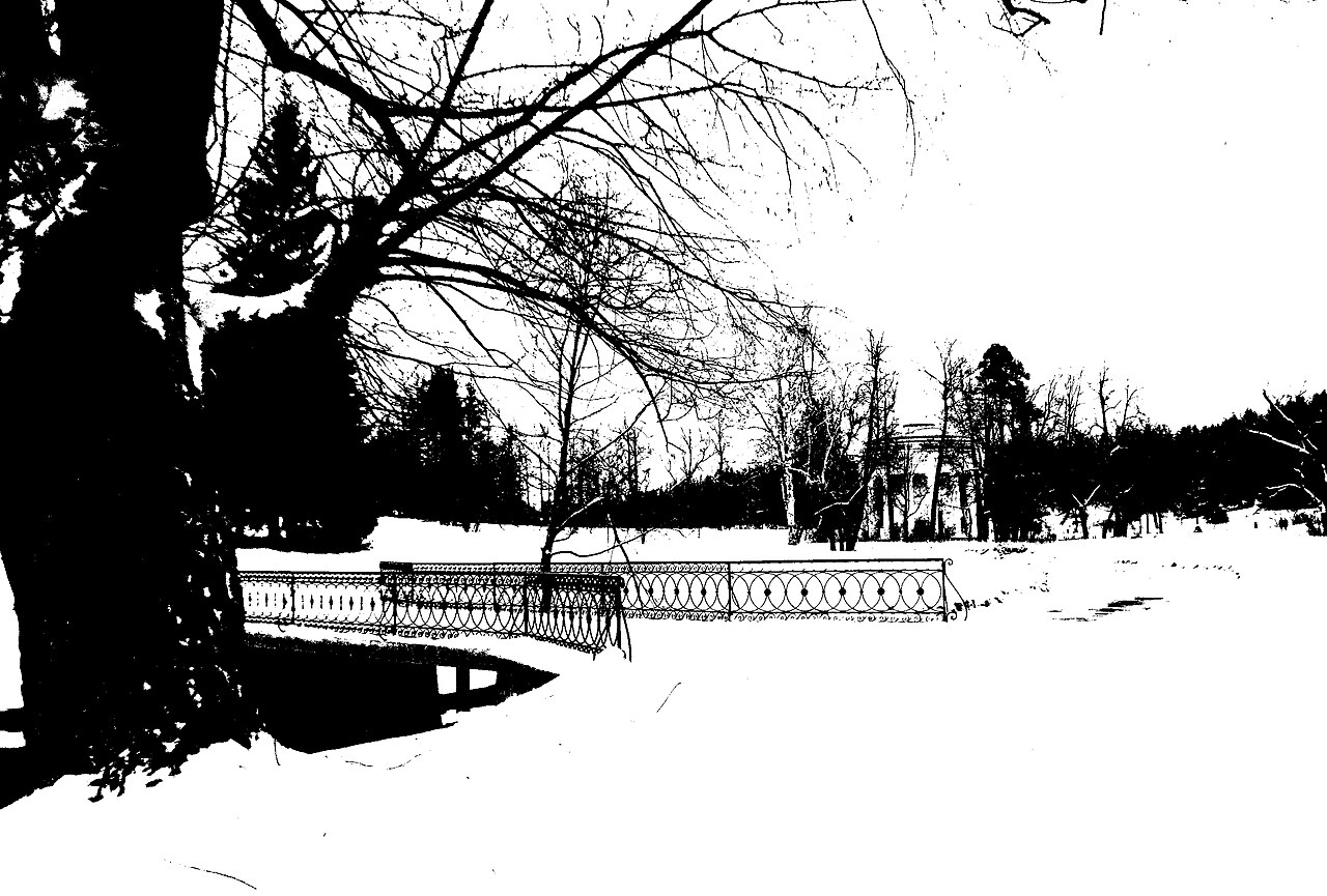
A photograph is a fog of grays. Ten thousand shades, none of them sure of itself, the railing bleeding into the snow, the snow bleeding into the sky.
Then you ask one question, the same question, of every single pixel: are you brighter than this line, or darker? Brighter goes white. Darker goes black. No maybes, no in-between.
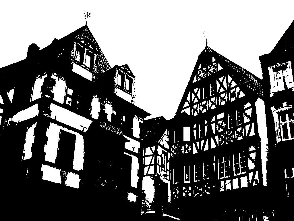
The fog snaps into a stencil. Thresholding is the moment an image stops describing the world and starts making a decision about it.
Before a computer can count cells, read a license plate, or trace the outline of a part on a conveyor belt, it usually needs to answer a much simpler question first: which pixels are thing, and which pixels are background? Thresholding is the bluntest, oldest, and still the most-used way to draw that line. You pick a brightness cutoff, call it , and every pixel votes itself into one of two camps. The result is a binary image: pure black and pure white, foreground and background, with nothing left to argue about.
Run the sim at the top of this page. Switch between Global, Otsu, and Adaptive, then drag the threshold slider slowly from one end to the other. Watch the blobs appear and dissolve. The thing to look for: the input has a deliberate left-to-right lighting gradient, so try to find a single slider value that cleanly recovers every dark blob on both the bright side and the shadowed side at once. You will not find one. That failure is the whole story of this chapter.
What you just felt is the tension at the heart of thresholding. A single global cutoff is a confident, brittle thing: it works beautifully when the lighting is even, and it falls apart the instant a shadow crosses the frame. Everything below is the slow, clever escape from that brittleness, from a hand-tuned slider, to a number the image picks for itself, to a different number for every neighborhood.
The one equation
For a grayscale image , global thresholding produces a binary image pixel by pixel:
Every symbol, in plain words:
- is the brightness of the input pixel at column , row , an integer from (black) to (white).
- is the threshold, the single cutoff you are choosing. It is the slider.
- is the output: (white, "foreground") if the pixel beats the cutoff, (black, "background") if it does not.
That is the entire operation. No convolution, no kernels, no calculus. It is the cheapest meaningful thing you can do to an image, which is exactly why it shows up at the front of so many pipelines.
Choosing T by hand, and why it hurts
The honest problem with the equation is that it does not tell you what should be. A photo of black ink on white paper has a beautiful answer: anywhere in the wide empty middle works. But most images are not that kind. Faces, landscapes, microscope slides, machined parts under a shop light: their brightness values smear across the whole range, and the "right" cutoff is a guess that you re-tune every time the lighting changes.
This is fragile in exactly the way that gets shipped to production and then breaks. A document scanner tuned in a bright office produces black-on-black garbage the moment someone scans under a desk lamp. The cutoff did not move; the world did.
Letting the image pick: Otsu's method
In 1979, a researcher at Japan's Electrotechnical Laboratory named Nobuyuki Otsu published a way to stop guessing. His insight: a good threshold should split the pixels into two groups that are each as internally consistent as possible. Pick the cutoff that makes the dark group tightly dark and the bright group tightly bright, and you have the most defensible line through the histogram.
Otsu's method turns threshold-picking into pure arithmetic on the histogram. It tries every possible cutoff, scores each one by how cleanly it separates the two groups, and keeps the winner. No human, no slider, no re-tuning when the camera moves. In the sim, the Otsu mode does exactly this: it reads the scene and reports back a single number.
Otsu's method is at its best when the histogram is bimodal, meaning it has two clear humps: one for the dark background, one for the bright foreground. The optimal cutoff lands in the valley between them.
But notice what Otsu still cannot do. It picks one number for the whole image. Point it at our gradient-lit blobs and it returns the statistically best global value, and that single value still loses to the shadow. Otsu solved which threshold; it did not solve one threshold for everything.
When one number is not enough: adaptive thresholding
The escape is to stop demanding a single answer. Adaptive thresholding computes a different cutoff for every pixel, based on the brightness of its immediate neighborhood:
In words: the threshold for a pixel is the average brightness of the small window around it (a plain mean, or a Gaussian-weighted one), minus a small constant that biases the decision toward background and kills speckle. Because each pixel is judged against its local surroundings, a dark blob in shadow is compared to other shadowed pixels, not to the sunlit half of the frame. The gradient stops mattering.
This is why Adaptive is the only mode in the sim that recovers every blob across the lighting gradient. It pays for that robustness with more computation (a moving average over the whole image) and a new knob, the window size, that must be larger than the things you want to keep but smaller than the lighting changes you want to ignore.
Beyond two camps
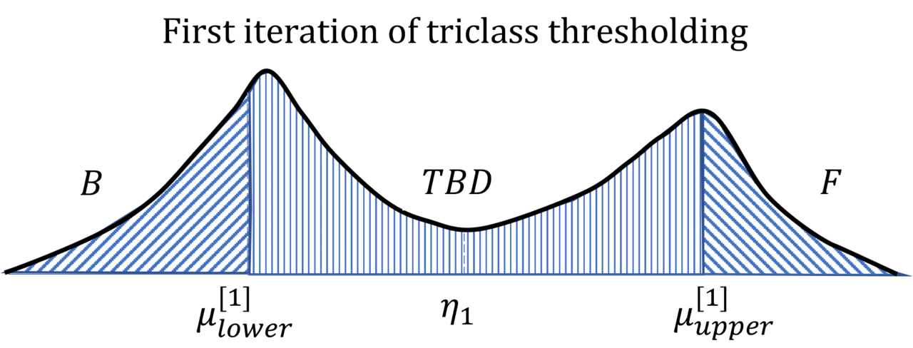
Why stop at black and white? The same separation logic extends to multi-level thresholding, slicing the histogram into three or more classes, which Otsu described in his original paper. More recent variants iterate the idea: threshold once, set aside the confidently-classified pixels, and re-threshold the uncertain middle, refining the boundary on each pass.
For the advanced reader → The math Otsu actually optimizes: within-class versus between-class variance
Otsu's method works on the normalized histogram. Let be the fraction of pixels with intensity , for (usually ). A candidate threshold splits the pixels into a background class (intensities ) and a foreground class (intensities ).
The class probabilities (the share of pixels in each camp) are:
and their mean intensities are:
Otsu wants the threshold that minimizes the within-class variance, the weighted spread inside the two groups:
Computing and for every candidate is expensive. Otsu's trick is that total variance is fixed, , so minimizing within-class variance is identical to maximizing the between-class variance:
That expression depends only on running sums of the histogram, so you sweep from to in a single linear pass and keep the that makes largest. It is, in modern terms, a globally optimal 1-D k-means on the intensity histogram, a discrete cousin of Fisher's linear discriminant. Beautifully cheap, and that cheapness is why it never went away.
Key takeaways
- Thresholding is the simplest segmentation: compare every pixel to a cutoff and emit pure black or pure white. It is fast, foundational, and feeds almost every higher-level pipeline.
- A hand-tuned global is brittle. It works under even lighting and shatters under shadows and gradients, because the cutoff stays put while the world's brightness wanders.
- Otsu's method (1979) lets the image choose by maximizing between-class variance, the cleanest split of a bimodal histogram, with no human in the loop.
- Adaptive thresholding beats uneven lighting by computing a local cutoff per pixel (), the only approach that survives the demo's gradient.
- Clean up first. Blur before thresholding to tame noise, and reach for multi-level methods when two camps are not enough.
Every threshold is a small act of certainty pressed onto an uncertain world. The fog of grays does not actually contain a sharp edge between thing and not-thing; we impose one, because decisions are cheaper than nuance and a stencil is easier to count than a cloud.
Otsu's gift was to make that act of certainty honest: not a number a tired engineer guessed at 2 a.m., but the line the histogram itself would draw if you asked it nicely. And when even one honest line is not enough, you simply ask the question again, neighborhood by neighborhood, until the shadow stops mattering. From a field of ten thousand grays, two answers, and the quiet confidence to commit to them.