Blob Detection
Finding Regions
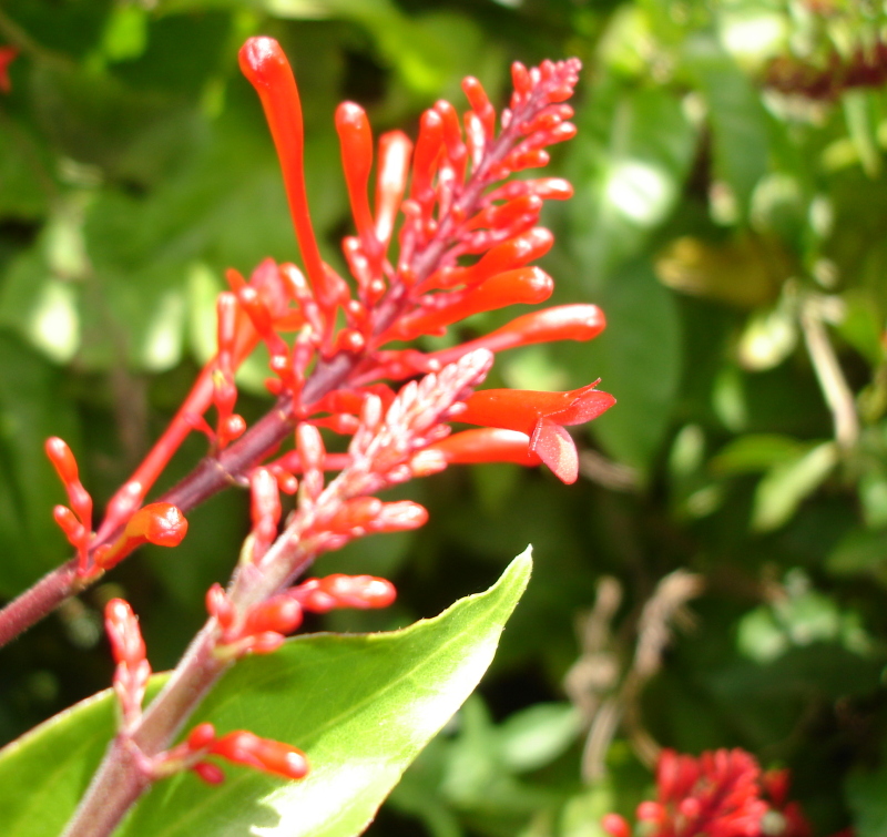
Squint at a photograph of the night sky and the stars stop being points. They swell into little smudges of light, each one a soft hill rising out of the dark. Squint at a microscope slide and the cells do the same: pale, rounded islands floating on a darker sea. Squint at a bag of coins on a table and every coin becomes a bright disc against the cloth.
Your eye is doing something a camera does not do for free. It is grouping pixels into things, deciding where one rounded patch ends and the background begins, all without anyone telling it what a star or a cell or a coin is.
A blob is a region of an image that stands apart from its surroundings, and finding blobs is how a computer learns to see objects before it knows their names.
Before a vision system can recognize a face or read a license plate, it has to answer a humbler question: where is there something here at all? Edge detectors trace the boundaries between regions, and corner detectors pin down sharp intersections, but neither tells you that a fat rounded patch of brightness is sitting in the middle of the frame. That is the job of blob detection: spotting compact regions where some property (usually brightness or color) is roughly constant inside and clearly different outside. A blob is the visual atom of "an object might be here."
Drag the min/max area and circularity sliders below and watch which regions survive the filter and which get rejected. Look for the moment when loosening the circularity bound suddenly lets ragged, non-round shapes through, and when tightening the area bound makes small specks vanish. Then tap 📷 Camera and point it at coins, buttons, or bubbles to see blobs flagged live.
What you just tuned is the difference between a candidate region and a kept detection. The detector proposes many bright or dark patches; the filters (area, circularity, convexity) are a set of cheap geometric tests that throw away the patches that do not look like the thing you care about. The art of blob detection is choosing those tests so that coins survive and reflections do not.
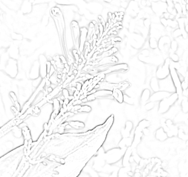
The cleanest mathematical definition of a blob comes from calculus. We treat the grayscale image as a function giving the brightness at each point, then look for places where the brightness curves away from its neighbors in every direction at once. The tool that measures that curvature is the Laplacian of a Gaussian:
Here is the image brightness at pixel ; is a Gaussian blur with standard deviation that controls how big a blob we are hunting for; the star is convolution (sliding the blur across the image); and is the Laplacian, the sum of the second derivatives, which is large in magnitude wherever the brightness is bending sharply. A bright blob on a dark background produces a strong negative LoG response right at its center, and that response is strongest when matches the blob's radius.
Two families: derivatives and extrema
Formally, blob detectors split into two camps. Differential methods take derivatives of the image (the LoG above is the classic example) and look for places where the curvature peaks. Extrema methods instead scan the image for local maxima and minima of some response function, treating each peak as a blob. The modern literature often folds both under the umbrella term interest point operators, because a blob, like a corner, is really just a location worth paying attention to.
The reason to bother at all is that blobs carry information edges and corners miss. An edge tells you there is a boundary here; a corner tells you two boundaries meet here; a blob tells you there is a coherent region of stuff here, about this big. That last fact, the size, turns out to be priceless. It lets a detector report not just where but at what scale, which is exactly what you need to match the same object in a close-up and a wide shot.
The scale problem, and the Gaussian trick
There is a catch hiding in the LoG equation: that little . A LoG tuned to find blobs of radius 5 pixels will shrug at a blob of radius 50. Real scenes contain objects at wildly different sizes, so a single-scale detector is nearly useless. The fix is to run the detector at many values of and keep the response that is strongest across both space and scale. This is scale-space: a stack of progressively blurrier versions of the image, one per , in which a blob shows up as a peak at the layer whose blur radius matches its size.
Computing a true Laplacian of Gaussian at every scale is expensive, so practitioners reach for a beautiful shortcut. Blur the image twice, with two nearby Gaussian widths, and subtract one result from the other. That difference of Gaussians (DoG) closely approximates the LoG while costing only two blurs and a subtraction:
Subtracting a more-blurred image from a less-blurred one keeps exactly the spatial detail that lives between the two blur radii and discards everything finer or coarser. In signal terms it is a band-pass filter: it passes a band of spatial frequencies and attenuates the rest. Structures whose size falls in that band light up; everything else fades to gray.
Why a Gaussian and not some other blur? Because the Gaussian is the unique kernel that creates no new detail as you increase . Blurring with it can only ever simplify the image, never invent a spurious bump, which means a blob that survives at a coarse scale is genuinely there and not an artifact of the smoothing. That guarantee, called scale-space causality, is the mathematical bedrock the whole approach stands on. The classic LoG profile even has a nickname: plotted in cross section it looks like a sombrero, so engineers call it the Mexican hat filter.

SIFT: the algorithm that ran on blobs for a decade
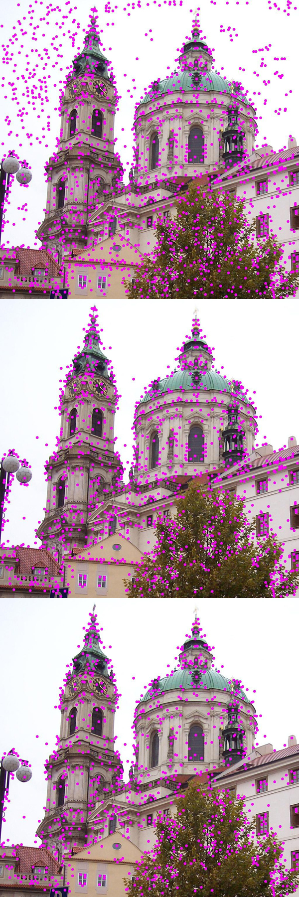
In 1999 a computer scientist named David G. Lowe, then a professor at the University of British Columbia, published an algorithm that would dominate computer vision for the next fifteen years: the Scale-Invariant Feature Transform, or SIFT. Its engine is exactly the scale-space difference of Gaussians described above. SIFT builds a pyramid of DoG images across many scales, finds the points that are local extrema in both space and scale (those are the blobs), and then attaches to each one a distinctive 128-number fingerprint describing the local gradients.
Because the keypoints are found in scale-space, they survive when the object is photographed closer or farther away, rotated, or partially hidden. That invariance made SIFT the workhorse behind object recognition, panorama stitching, 3D reconstruction, robot navigation, and even individual identification of wild animals from their markings. Match the fingerprints between two images, cluster the matches that agree on a consistent pose using a Hough transform, verify, and you have recognized an object with high confidence.
From theory to a practical pipeline
You rarely need full SIFT just to count coins. A simple blob detector, like the one driving the demo at the top, follows a pragmatic recipe:
- Threshold the grayscale image at several levels to produce binary masks.
- Find connected components, the groups of touching pixels, in each mask.
- Filter by geometry, keeping only components that pass area, circularity, and convexity tests.
The most intuitive of those tests is circularity, a single number that asks "how round is this region?"
where is the blob's area in pixels and is the length of its perimeter. The constant is chosen so that a perfect circle scores exactly . A square comes out to about , and a long thin streak drives the perimeter up while the area stays small, sending toward . Set a minimum circularity and you have a cheap, rotation-invariant filter that keeps coins and rejects scratches.
Why a circle maximizes circularity, and where the 4π comes from
The formula is the isoperimetric inequality in disguise. For any closed plane curve enclosing area with perimeter ,
with equality only for a circle. Rearranged, that says
so is the ceiling and a circle is the unique shape that reaches it. To see where the constant comes from, plug in a circle of radius : its area is and its perimeter is , so
The is precisely the factor that normalizes the circle to one. Two warnings for real images. First, perimeter is brutal to measure on a pixel grid: a staircased boundary inflates , dragging below 1 even for genuinely round blobs, so practical detectors use a forgiving threshold like rather than demanding . Second, circularity says nothing about whether a shape is convex: a five-pointed star and a pentagon can share a circularity score, which is why convexity (the ratio of a blob's area to the area of its convex hull) is tracked as a separate filter.
Key takeaways
- A blob is a compact region where some property is roughly constant inside and different outside. It is the visual unit of "an object might be here," carrying information that edges and corners cannot.
- The Laplacian of Gaussian measures blob-ness as curvature. Its response peaks when the blur scale matches the blob's radius, which is why blob detection is inseparable from the question of scale.
- Difference of Gaussians is the cheap, accurate stand-in for LoG. Two blurs and a subtraction give a band-pass filter that keeps mid-scale structure and discards the rest, mirroring the center-surround cells in your own retina.
- SIFT, built on scale-space DoG blobs, ran computer vision for fifteen years. David Lowe's 1999 algorithm gave keypoints that survive scaling, rotation, and occlusion; its patent expired in 2020.
- Circularity is a one-line roundness test, bounded above by 1 (the circle) thanks to the isoperimetric inequality, and paired with area and convexity to turn raw candidate regions into trustworthy detections.
We began by squinting at stars and cells and coins, watching them swell into soft hills of light. That swelling is not an accident of tired eyes; it is the very signature a blob detector hunts for, a region of brightness curving away from the dark in every direction at once.
Teach a machine to find those hills at every scale and you have given it the first, wordless act of seeing: not what is there, but simply that something is. From that humble spark, a patch of pixels deemed worth a second look, grows everything else, the recognizing, the matching, the naming.