🎯 Corner Detection

The whole field calls these spots interest points or feature points, and corner detection is the craft of finding them automatically. The intuition is almost embarrassingly simple: a good feature is one you could not have found anywhere else. A patch of blue sky could be any patch of blue sky. A stretch of brick wall slides into the next stretch. But the precise junction where two lines cross is a fingerprint. Track that fingerprint across two photos and you have tied them together.

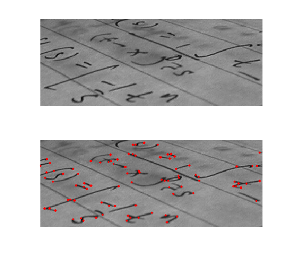
Drag the corner threshold in the sandbox below and flip the output between the Harris response heatmap and the detected Corners, then tap 📷 Camera and aim it at a checkerboard or a window frame. Look for where the heatmap glows brightest: not along the clean edges, but at the intersections where edges collide.

What the heatmap reveals is that "edge" and "corner" are not the same animal. Edges light up faintly and stretch out in lines; corners flare into bright isolated dots. The detector is scoring every pixel by a single question: if I shifted my little window away from here, in every direction, how violently would the picture underneath change? Flat regions score near zero. Edges score high in one direction and low in the other. Corners score high all around. That triage, flat versus edge versus corner, is the engine of everything that follows.

The aperture problem

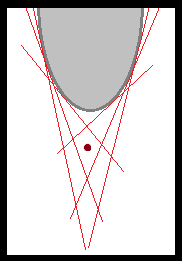
Look at the world through a soda straw and try to judge which way a tilted line is moving. You cannot. You only ever see the line cross your tiny circle of view, so motion along the line is invisible. This is the aperture problem, and it is the reason edges make terrible features. Through a small window, an edge can slide endlessly without announcing it.

We can make this precise. Take a small image window $W$ and ask how much its contents change if we shift it by $(u, v)$. The sum of squared differences is:

$E(u, v) = \sum_{(x,y) \in W} \bigl[\, I(x+u,\, y+v) - I(x, y) \,\bigr]^2$

Here $I(x,y)$ is the image brightness at pixel $(x,y)$, the pair $(u,v)$ is the small shift we test, and $W$ is the window of pixels we sum over. $E$ measures the total change the shift causes. A flat patch gives $E \approx 0$ for every shift. An edge gives $E \approx 0$ for shifts along it. Only a corner gives a large $E$ in all directions, and that is exactly the "lurch" you felt in the Hook.

The Harris corner detector

In 1988 Chris Harris and Mike Stephens, working on motion analysis in Plessey's research labs in Britain, took Moravec's idea and made it smooth. Instead of physically shifting the window in a handful of clumsy directions, they used calculus. A first-order Taylor expansion of $E(u,v)$ turns that messy sum into clean linear algebra, and out drops a small matrix that encodes the local image structure in every direction at once:

$M = \sum_{W} \begin{bmatrix} I_x^2 & I_x I_y \\ I_x I_y & I_y^2 \end{bmatrix}$

where $I_x$ and $I_y$ are the image gradients (how fast brightness changes left-to-right and top-to-bottom, usually computed with a Sobel filter), and the sum runs over the window $W$. This $2 \times 2$ matrix $M$ is called the structure tensor. Its two eigenvalues, $\lambda_1$ and $\lambda_2$, tell you how strongly the image varies along the two principal directions of the window. Two small eigenvalues mean a flat region; one large and one small mean an edge; two large eigenvalues mean a corner.

Computing eigenvalues at every pixel was expensive in 1988, so Harris and Stephens used a clever shortcut. They scored each pixel with:

$R = \det(M) - k \cdot \operatorname{trace}(M)^2$

The trick is that $\det(M) = \lambda_1 \lambda_2$ and $\operatorname{trace}(M) = \lambda_1 + \lambda_2$, so $R$ can be read straight off the matrix without ever solving for the eigenvalues. The constant $k$ is an empirical fudge factor, usually between $0.04$ and $0.06$. A large positive $R$ means a corner, a large negative $R$ means an edge, and $R$ near zero means a flat region. That is precisely the heatmap you scrubbed through above.

Shi-Tomasi and the honest minimum

Six years later, in 1994, Jianbo Shi and Carlo Tomasi asked a sharper question: not "what is a corner?" but "what is a feature good to track?" Their answer dropped Harris's clever determinant shortcut and went back to the eigenvalues themselves. They scored each pixel by:

$R = \min(\lambda_1, \lambda_2)$

The reasoning is plainly stated once you see it. A point is only trackable if it changes strongly in every direction, and the weakest direction is the one set by the smaller eigenvalue. So score the point by its weakest link. If even the minimum eigenvalue is large, the point is solid in all directions. This Shi-Tomasi measure proved more stable in practice and became the default behind OpenCV's goodFeaturesToTrack().

There is one more idea you need before the corners are usable. A strong corner does not light up a single pixel; it lights up a small bright blob of high response. Left alone, the detector would report the same corner a dozen times over. Non-maximum suppression fixes this: scan for local maxima of $R$, and within each neighborhood keep only the single strongest response, discarding its dimmer neighbors. The result is the clean scatter of well-separated points you want to feed into a tracker.

↘ For the advanced reader → Where the structure tensor M actually comes from

Start from the change function and Taylor-expand the shifted image to first order:

$I(x+u,\, y+v) \approx I(x,y) + I_x\, u + I_y\, v$

Substitute that into $E(u,v)$ and the $I(x,y)$ terms cancel, leaving a sum of squared linear terms:

$E(u, v) \approx \sum_W \bigl( I_x\, u + I_y\, v \bigr)^2$

Expand the square and group the $u$ and $v$ coefficients, and the whole expression collapses into a quadratic form:

$E(u, v) \approx \begin{bmatrix} u & v \end{bmatrix} \, M \, \begin{bmatrix} u \\ v \end{bmatrix}, \qquad M = \sum_W \begin{bmatrix} I_x^2 & I_x I_y \\ I_x I_y & I_y^2 \end{bmatrix}$

This is the punchline of the Harris derivation. The change in any direction is governed entirely by the structure tensor $M$. The eigenvectors of $M$ point along the directions of greatest and least change, and the eigenvalues $\lambda_1, \lambda_2$ give their magnitudes. The surface $E$ is a bowl whose steepness is set by those eigenvalues:

• Both small: a shallow, near-flat bowl. Flat region.
• One large, one small: a long trough. Edge (free to slide along the trough).
• Both large: a steep, isotropic bowl. Corner.

Harris's $R = \lambda_1 \lambda_2 - k(\lambda_1 + \lambda_2)^2$ and Shi-Tomasi's $R = \min(\lambda_1, \lambda_2)$ are just two different ways of squeezing this two-eigenvalue situation into a single trackability score.

Key takeaways

• A corner is a point that changes in every direction. Flat regions are ambiguous, edges suffer the aperture problem, only corners are unique enough to track and match.
• The structure tensor $M$ is the whole machine. Built from squared image gradients summed over a window, its two eigenvalues classify each pixel as flat, edge, or corner.
• Harris (1988) scores cheaply with $R = \det(M) - k\,\operatorname{trace}(M)^2$, avoiding an explicit eigenvalue solve while sorting corners, edges, and flats in one pass.
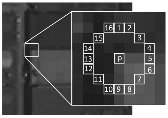
• Shi-Tomasi (1994) scores with $\min(\lambda_1, \lambda_2)$, asking directly "is this good to track?" and is the default behind OpenCV's goodFeaturesToTrack().
• Non-maximum suppression turns blobs of response into clean points, and FAST (2006) trades gradient math for a ring test to hit real-time speeds.