✨ Noise Reduction

Every image carries a layer of noise: random jitter in brightness or color that has nothing to do with the scene. It rides in with the shot noise of counting photons, with the heat in the sensor's circuitry, with the compression that squeezes a file down. Our job is to smooth that randomness away while leaving the real structure (edges, textures, faces) standing. The catch is that noise and detail can look alike up close, so every smoothing method is a negotiation, not a cure.

Drag the blur radius slider in the simulator at the top of this lesson. At radius zero you see the raw, speckled frame. As you push the radius up, watch two things at once: the random fizz melts away, but the clean edge of the disc also goes soft. Then tap 📷 Camera, point it at a flat wall, and see the live grain dissolve under your finger.

That softening is the whole story in miniature. Averaging neighbors kills randomness because the random parts cancel, but it also averages across the genuine boundaries you wanted to keep. The rest of this chapter is a tour of filters that try to win back the edges.

The Gaussian blur: a weighted vote

The simplest smoother replaces each pixel with the average of its neighbors. A Gaussian blur is the polished version: instead of weighting every neighbor equally, it weights them by a bell curve, so a pixel right next door counts far more than one three steps away. The result is a soft, natural smoothing, like viewing the scene through frosted glass.

In one dimension the weight at distance $x$ from the center is

$G(x) = \frac{1}{\sqrt{2\pi}\,\sigma}\, e^{-\frac{x^2}{2\sigma^2}}$

where $x$ is the offset from the pixel you are filtering, $\sigma$ (sigma) is the standard deviation that sets how wide the bell is (a bigger $\sigma$ reaches further and blurs harder), $e$ is Euler's number, and the $\tfrac{1}{\sqrt{2\pi}\,\sigma}$ in front is a normalizing factor so the weights sum to one and the image keeps its overall brightness.

For an image you use the 2D version, which is just two of these multiplied together. In practice we sample it into a small integer kernel and slide it over the picture:

$K = \frac{1}{273}\begin{bmatrix} 1 & 4 & 7 & 4 & 1 \\ 4 & 16 & 26 & 16 & 4 \\ 7 & 26 & 41 & 26 & 7 \\ 4 & 16 & 26 & 16 & 4 \\ 1 & 4 & 7 & 4 & 1 \end{bmatrix}$

The center pixel gets the heaviest weight ($41/273$), the corners the lightest ($1/273$), and dividing by $273$ (the sum of all the entries) keeps the brightness honest.

The Gaussian's pros and cons are two sides of one coin. It is smooth and well behaved, with no ringing or overshoot, and it has a beautiful trick: a 2D Gaussian is separable, meaning you can blur all the rows and then all the columns instead of doing the full 2D sum. That turns a costly operation into two cheap ones. The downside is blunt honesty: it cannot tell a noisy edge from a clean one, so it blurs your boundaries right along with the grain.

The median filter: throw out the outliers

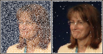
Some noise is not a gentle fuzz but a violent one. Salt-and-pepper noise scatters pure-white and pure-black pixels across the frame, the kind of damage you get from a flaky sensor or a bad transmission. Averaging is the worst possible response: a single white speck of value 255 drags the whole neighborhood's average upward, smearing the corruption instead of removing it.

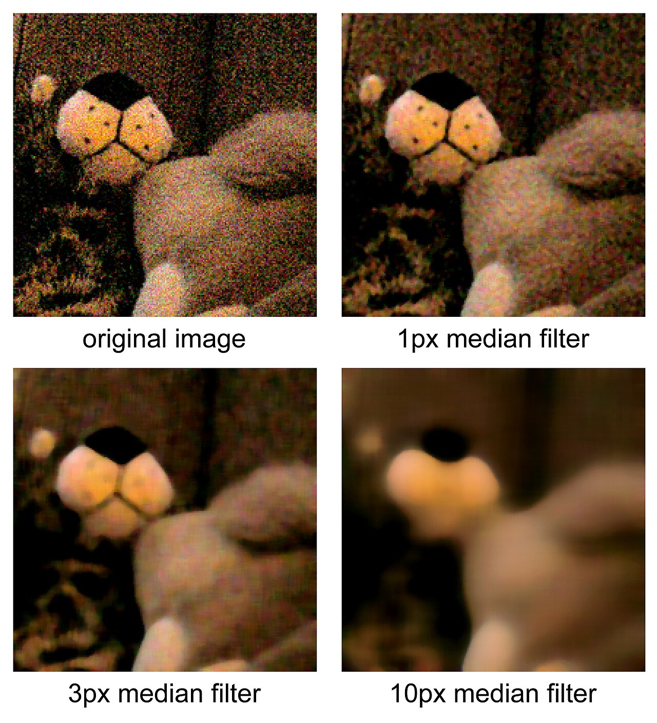
The median filter sidesteps this entirely. Instead of averaging, it sorts. For each pixel it gathers the neighborhood, lines up all the values in order, and picks the one in the middle:

$I'(x, y) = \operatorname{median}\bigl\{\, I(i, j) : (i, j) \in \mathcal{N}(x, y) \,\bigr\}$

Here $I'(x,y)$ is the cleaned pixel, $I(i,j)$ are the original values, and $\mathcal{N}(x,y)$ is the neighborhood window (a $3 \times 3$ block, say) around the pixel. The median ignores extreme outliers by construction: a lone white speck sits at the far end of the sorted list and never gets chosen. Better still, on a clean edge most of the window already shares one value, so the median keeps the edge crisp where a Gaussian would have smudged it.

Because the median is a non-linear operation (you cannot get it by adding scaled copies of the input), it does things no convolution kernel can. It is the standard pre-processing step before edge detection precisely because it strips impulse noise while leaving the boundaries that edge detectors hunt for. The cost is that very fine detail, thin lines and small dots barely wider than the window, can be voted away as if they were noise.

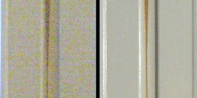
The bilateral filter: smoothing that respects edges

What if we could have the Gaussian's smoothness and the median's respect for edges? That is the promise of the bilateral filter, and it earns it with one clever idea: weight neighbors by two things at once, not one.

A plain Gaussian asks a single question of each neighbor: how far away are you? The bilateral filter asks a second: how different is your brightness from mine? A neighbor that is both close in space and close in color gets full vote. A neighbor that sits just across a sharp edge, near in space but very different in brightness, gets almost no vote at all. The filter smooths happily inside flat regions but refuses to average across boundaries, because the pixels on the far side simply do not count.

$I'(p) = \frac{1}{W_p} \sum_{q \in \mathcal{N}} G_s\bigl(\lVert p - q \rVert\bigr)\, G_r\bigl(\lvert I(p) - I(q) \rvert\bigr)\, I(q)$

Read it left to right: $I'(p)$ is the new value at pixel $p$; the sum runs over each neighbor $q$; $G_s$ is the spatial Gaussian that fades with distance $\lVert p - q \rVert$; $G_r$ is the range Gaussian that fades with the brightness difference $\lvert I(p) - I(q) \rvert$; their product is the weight; and $W_p$ is the sum of all those weights, dividing through so brightness is preserved. Knock out $G_r$ and you are left with an ordinary Gaussian blur. That extra factor is the entire difference between a filter that blurs edges and one that guards them.

The price is speed. Because the range weights depend on the actual pixel values, the bilateral filter is not separable: you cannot split it into a row pass and a column pass the way you can a Gaussian, so the naive version is markedly slower. Whole research papers exist just to approximate it fast enough for video.

↘ For the advanced reader → Why the Gaussian is the only blur with no ringing

The Gaussian is special among smoothing kernels, and the reason lives in the frequency domain. Convolving an image with a kernel multiplies its frequency content by the kernel's transfer function. The remarkable fact is that the Fourier transform of a Gaussian is itself a Gaussian:

$\mathcal{F}\bigl\{ e^{-x^2 / 2\sigma^2} \bigr\}(\omega) \;\propto\; e^{-\sigma^2 \omega^2 / 2}$

A Gaussian in space maps to a Gaussian in frequency, and a Gaussian is positive everywhere with no oscillation. So the filter rolls high frequencies off smoothly and monotonically, never letting any band overshoot. A box (simple-average) blur, by contrast, has a transfer function that is a sinc, which wobbles above and below zero, and those wobbles are the visible ringing artifacts you see around hard edges after a crude blur.

There is a deeper trade-off underneath. A function and its Fourier transform cannot both be arbitrarily narrow: their spreads obey

$\Delta x \cdot \Delta \omega \;\geq\; \tfrac{1}{2},$

the same uncertainty principle that governs quantum mechanics. The Gaussian is the unique function that achieves equality, the single shape that is as compact as physically possible in space and frequency at once. That is why a Gaussian filter gives the best simultaneous suppression of high frequencies and the tightest spatial footprint: it sits exactly at the boundary the mathematics allows.

The separability that makes it fast is its other gift. Because $e^{-(x^2 + y^2)/2\sigma^2} = e^{-x^2/2\sigma^2} \cdot e^{-y^2/2\sigma^2}$, a 2D Gaussian factors into two 1D Gaussians, turning an $O(n^2)$ kernel into two $O(n)$ passes. No other rotationally symmetric blur factors so cleanly.

Choosing a filter

There is no universal winner; each filter is matched to a kind of noise.

| Filter | Speed | Edge preservation | Salt-and-pepper | |---|---|---|---| | Gaussian | Fast (separable) | Poor | Poor | | Median | Medium | Good | Excellent | | Bilateral | Slow | Excellent | Good |

Reach for the Gaussian when you want a quick, general smoothing or a pre-blur ahead of edge detection. Reach for the median when the damage is impulsive, the lone white and black specks of a glitchy sensor. Reach for the bilateral when edges matter most and you can spare the cycles. Most real pipelines use more than one in sequence.

Key takeaways

• Noise is intrinsic, not accidental. Shot noise, sensor heat, and compression all inject random variation; it is the unavoidable cost of measuring light, and it rides in with every frame.
• All smoothing is a trade-off between killing noise and preserving detail. Average over a wider neighborhood and more grain cancels, but more genuine edges blur too.
• The Gaussian is the smooth default, weighting neighbors by a bell curve. It is separable (hence fast) and ring-free, but blind to edges.
• The median filter is non-linear and outlier-proof, the right tool for salt-and-pepper noise, and it keeps edges crisp because it sorts rather than averages.
• The bilateral filter weights by space and color together, so it smooths flat regions while refusing to blur across boundaries, at the cost of speed.