Edge Detection
Finding Boundaries
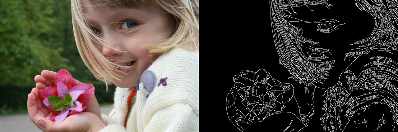
A child holds out a fistful of pink flowers. Now throw away the color. Throw away the soft shading on her cheek, the warm light in her hair, the green blur of the garden behind her. Keep only the places where the picture changes suddenly: the rim of a petal, the edge of a sleeve, the line of a smile.
What is left is a tangle of thin white lines on black. And yet you still see a girl, still see flowers, still read the whole scene in an instant. You threw away almost every number in the image and lost almost no meaning.
An edge is where the image changes sharply, and edges carry the lion's share of what a picture means.
The trick a vision system pulls here is older than computers. An edge is just a place where brightness jumps: dark fabric against a bright face, a petal against shadow. Our eyes are wired to chase exactly these jumps, which is why a four-line cartoon of a face is unmistakably a face. Edge detection is the act of teaching a machine to find those jumps and nothing else, turning a dense grid of pixels into a sparse sketch of boundaries.
The demo at the top of this page builds that sketch in front of you. Drag the threshold slider, flip the output between Gradient and Edges, then tap 📷 Camera and watch your own outline appear live beside the real feed. Look for the moment when raising the threshold erases the noise and faint texture first, leaving only the strongest contours standing. That is the central tension of edge detection in one slider: too low and you drown in spurious edges, too high and real boundaries vanish. The continuous Gradient view shows the raw evidence; the Edges view shows the verdict after a cutoff.
An edge is a steep slope
Picture a single row of the image as a landscape, where bright pixels are high ground and dark pixels are valleys. Across a flat wall the landscape is level. At the boundary of an object it drops off a cliff. The steepness of that cliff is the gradient, and a steep gradient means an edge.
In calculus the steepness of a function is its derivative. An image has two directions to vary in, so it has two partial derivatives, and together they form the gradient vector:
Here is the image brightness at a pixel. is how fast brightness changes as you step sideways (it lights up at vertical edges). is how fast it changes as you step downward (it lights up at horizontal edges). The two together point in the direction of steepest increase. We usually care about two summary numbers built from them:
The magnitude is how strong the edge is (the height of the cliff), written with the shorthand and . The direction is which way the cliff faces, an angle pointing across the edge rather than along it. The demo at the top computes exactly this magnitude on a synthetic scene, an uploaded photo, or your live camera, then keeps every pixel above the threshold.
Measuring the slope with Sobel
You cannot take a true derivative of a pixel grid (it has no smooth formula), so you estimate the slope from neighbors. The classic estimator is the Sobel operator: two small 3×3 kernels, slid across the image by convolution (the operation from the previous lesson), that approximate and .
Gx (vertical edges)      Gy (horizontal edges)
[-1  0  +1]              [-1  -2  -1]
[-2  0  +2]              [ 0   0   0]
[-1  0  +1]              [+1  +2  +1]
Notice the structure. The kernel subtracts the left column from the right column: if they differ, brightness is changing left-to-right, so there is a vertical edge. The middle row gets double weight, which quietly blurs along the edge while differencing across it, making the estimate less jittery in noise. Each kernel sums to zero, so a flat region (every neighbor equal) returns exactly zero. Only change survives.
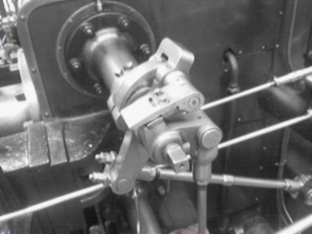
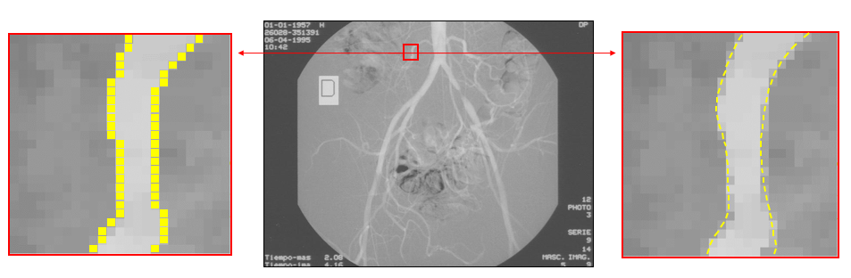
Run Sobel on an image like the valve above and you get the raw Gradient view from the demo: bright where rims and rods cut against their background, dark across flat castings. But raw gradients are fat and fuzzy. A single physical edge produces a thick smear of high-gradient pixels because the cliff has finite width and the image has noise. A good detector still has work to do: it must decide which of those pixels are the edge.
Canny: turning evidence into a verdict
In 1986 a graduate student named John Canny asked a sharper question than "where are the gradients?" He asked what an optimal edge detector would even mean, and answered it with three goals: catch every real edge (good detection), place each edge exactly (good localization), and mark each edge once, not as a thick band (single response). From those criteria he derived an algorithm that is still the gold standard four decades later. The Canny edge detector runs five stages:
- Gaussian blur to suppress noise, so the detector chases real cliffs, not speckle.
- Sobel gradients to measure magnitude and direction at every pixel.
- Non-maximum suppression to thin each fat ridge down to a one-pixel line, keeping only the pixel that is a local maximum across the edge.
- Double threshold to sort pixels into strong, weak, and discarded by two cutoffs instead of one.
- Hysteresis to keep a weak edge only if it touches a strong one, linking faint contours into the bold ones they belong to.
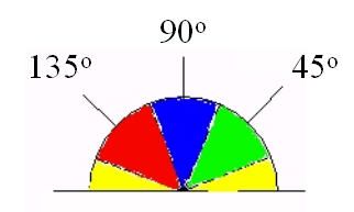
Stage 3 is where edge detection gets clever, and the demo's threshold control gives you a feel for stages 4 and 5. To suppress non-maxima you need the gradient direction, , which you snap to the nearest of four orientations (horizontal, vertical, and the two diagonals) so you can ask the simple question: is this pixel brighter in gradient than its two neighbors along ? If not, it is on the shoulder of the cliff, not the peak, and gets zeroed. That is how a smear becomes a line.
The double threshold then replaces the single slider with two. Pixels above the high threshold are certainly edges. Pixels below the low threshold are certainly not. The interesting ones lie between: weak candidates that hysteresis keeps only if a chain of pixels connects them back to a strong, confident edge. This is why a faint contour that trails off a bold one survives, while an isolated speck of noise of the same strength does not. Drag the demo's threshold and you are watching a one-dimensional version of this decision: every pixel of evidence judged against a cutoff.
Reading the edges back out
A clean edge map is rarely the final product; it is raw material. Stack subpixel fitting on top and you can locate a boundary to a fraction of a pixel, which matters enormously in measurement.
That precision is why edge detection quietly powers so much: lane lines for self-driving cars, the paper boundary your phone snaps to when it scans a document, the outline of a tumor in a radiograph, the silhouette that a robot arm uses to grasp a part. In each case the pipeline is the same shape you have been dragging in the demo: find the gradient, decide on a threshold, keep the boundaries, discard the rest.
For the advanced reader → Why a Gaussian first, and how blur and differentiation fold into one kernel
Differentiation amplifies noise. A derivative measures change, and noise is change, so running Sobel on a raw image makes every speck of sensor grain shout. Canny's first stage answers this by smoothing with a Gaussian of standard deviation :
The beautiful part is that you never need two passes. Convolution is associative and the derivative is linear, so differentiating the blurred image equals convolving once with the derivative of the Gaussian:
So blur-then-difference collapses into a single oriented kernel applied once. Choosing trades detection against localization: a large smooths away noise but rounds off corners and shifts edges, while a small pins edges precisely but lets noise through. That trade-off is exactly the tension you feel in the demo's threshold, pushed one stage earlier into the blur.
Marr and Hildreth took the second-derivative route instead. Their operator is the Laplacian of Gaussian,
and edges are the zero crossings of . An edge is a peak in the first derivative, which is the same as a zero crossing in the second derivative, so both schools are looking at the same cliff from two sides of the calculus.
Key takeaways
- An edge is a steep gradient. Brightness changing sharply over a short distance is the entire signal; everything else can be thrown away with surprisingly little loss of meaning.
- The gradient has a magnitude and a direction. says how strong the edge is; says which way it faces.
- Sobel estimates the slope by convolution. Two zero-sum 3×3 kernels difference across the edge while averaging along it, so flat regions vanish and only change survives.
- Canny turns evidence into a verdict. Blur, gradient, non-maximum suppression, double threshold, and hysteresis together catch real edges, place them precisely, and mark each one exactly once.
- Thresholds are a trade-off, not a setting. Too low drowns you in noise, too high erases real boundaries; hysteresis softens the choice by linking weak edges to strong neighbors.
Edge detection is, in the end, an act of forgetting done well. The girl with her flowers survives being reduced to a fistful of white lines because the lines were never decoration; they were where the meaning lived all along.
Every detector since, from Sobel's lab folklore to Canny's optimal criteria, is a refinement of one ancient instinct your own eyes obey before you are even aware of looking: find where the world changes, and there you will find its shape.