🔲 Convolution

The stencil is called a kernel (you will also see it called a filter, a convolution matrix, or a mask). It is usually a tiny square: 3x3, sometimes 5x5. The numbers inside it decide what the operation does. Change the weights and the same machinery becomes a different tool: average the neighbors and you get blur; subtract the neighbors and you get edges. The image never changes its nature. Only the kernel does.

Open the sandbox below and load the Sobel X preset, then flip the output canvas between your input and the result. What to look for: flat regions (a clear sky, a painted wall) collapse to black, while every boundary lights up. Now load Blur and watch fine detail dissolve into a soft haze. The debrief: a kernel whose weights sum to one preserves brightness (blur, identity), while a kernel whose weights sum to zero throws away the flat parts and keeps only change (every edge detector). That single bit of arithmetic, what the weights add up to, predicts what the filter will do before you ever run it.

The governing equation

For a kernel $K$ of size $(2a{+}1)\times(2b{+}1)$ centered on each pixel, the filtered image $G$ is

$$G(x, y) = \sum_{i=-a}^{a} \sum_{j=-b}^{b} K(i, j)\, \cdot\, I(x - i,\; y - j)$$

Reading it in plain words:

• $I(x, y)$ is the input image: the brightness of the pixel at column $x$, row $y$.
• $G(x, y)$ is the output pixel you are computing, at the same location.
• $K(i, j)$ is the weight at offset $(i, j)$ inside the kernel, with $(0,0)$ at its center.
• The double $\textstyle\sum$ just says "visit every cell of the kernel, multiply, and total it up."
• The minus signs ($x - i$, $y - j$) are the famous flip: convolution reflects the kernel before sliding it. Reach the right edge of the kernel and you read the left edge of the image patch. (More on why this matters below.)

That is it. One weighted sum, repeated at every pixel. The art is entirely in choosing $K$.

The kernel is the personality

A kernel is a small matrix used for blurring, sharpening, embossing, edge detection, and more. Three classics show the pattern clearly.

The box blur averages its neighbors, smearing out noise:

$$K_{\text{blur}} = \frac{1}{9}\begin{bmatrix} 1 & 1 & 1 \\ 1 & 1 & 1 \\ 1 & 1 & 1 \end{bmatrix}$$

Its nine weights sum to $1$, so a flat patch stays exactly as bright as before. Sharpening does the opposite: it amplifies the gap between a pixel and its surroundings.

$$K_{\text{sharpen}} = \begin{bmatrix} 0 & -1 & 0 \\ -1 & 5 & -1 \\ 0 & -1 & 0 \end{bmatrix}$$

And the Sobel X operator, the star of the next lesson, subtracts the left column from the right to estimate how fast brightness changes horizontally:

$$K_{\text{sobel}} = \begin{bmatrix} -1 & 0 & 1 \\ -2 & 0 & 2 \\ -1 & 0 & 1 \end{bmatrix}$$

Its weights sum to $0$. On a flat region (left and right equal), the answer is exactly zero, so flat goes black. Only where the two sides disagree, an edge, does anything survive.

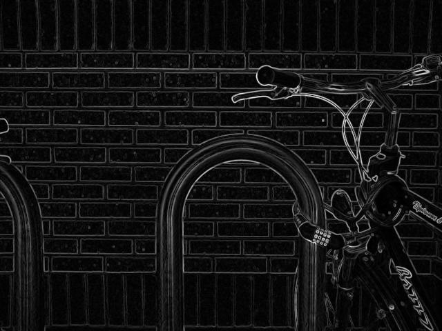
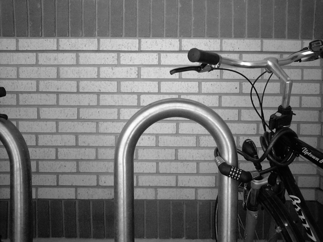
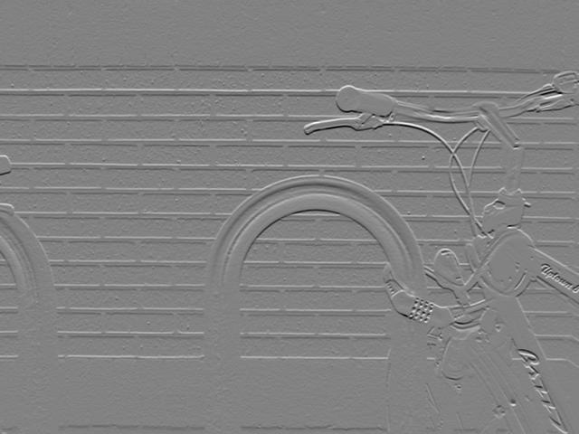
You can see the personalities side by side on a single test image. Below, the same grayscale bicycle is run through three different kernels.

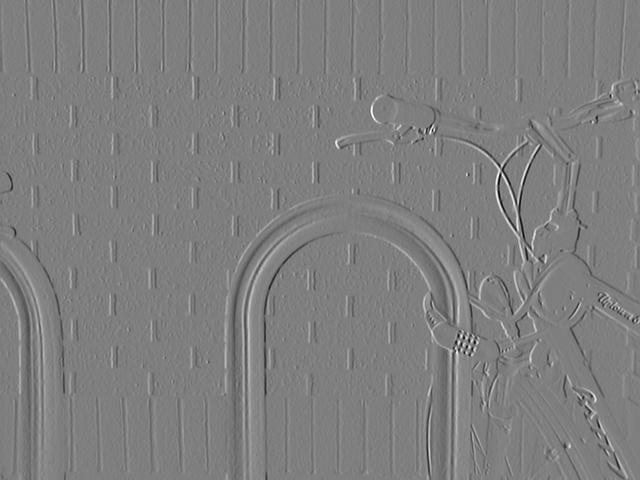
The Sobel operator is separable and integer-valued, which makes it cheap to compute, and at each point it gives you a gradient vector. Combine $G_x$ and $G_y$ and you get the full edge map from the chapter's hero image. The gradient approximation it produces is admittedly crude, especially for fine, high-frequency texture, but it is fast, robust, and good enough that it has outlived nearly every fancier alternative.

What happens at the border

Slide a 3x3 kernel onto the very first pixel of an image and you have a problem: there is nothing to the left of it, and nothing above it. The kernel hangs off the edge. Every convolution must decide what to read in that empty space, and the choice quietly changes the result along every border. The common strategies:

• Zero padding: pretend the off-image pixels are black ($0$). Simple, but it darkens the edges and can fake an edge where the image just stops.
• Replicate: extend the nearest border pixel outward. The corner stretches into the void.
• Reflect: mirror the image across its own edge, as if a mirror stood at the boundary. Usually the most natural-looking choice.
• Wrap: treat the image as a torus, where the right edge meets the left. Useful for tileable textures, strange for photos.

OpenCV exposes all four (and more) as the borderType argument to cv2.filter2D and cv2.copyMakeBorder. It is the kind of detail you ignore until a thin bright halo appears around every processed frame, and then you remember it forever.

Why "convolution" reaches far beyond images

The word predates computers by more than a century. In mathematics, convolution is an operation on two functions $f$ and $g$ that produces a third function, written $f * g$, as the integral of their product after one of them is reflected and then slid past the other. It expresses, in a single number for each shift, how much the shape of one function is modified by the other.

That abstract definition is why the same idea shows up in probability (the distribution of a sum of two random variables is the convolution of their distributions), in acoustics and audio (reverb is your dry signal convolved with the impulse response of a room), in optics (a blurry photo is the sharp scene convolved with the lens's point-spread function), and in signal processing (every finite-impulse-response filter is a convolution). An image filter is just this universal operation specialized to a 2D grid of pixels.

And it is why blurring an image is literally the optical-blur story made digital. Run a Gaussian kernel over a sharp scene and you reproduce, in software, exactly what an out-of-focus lens does in glass.

↘ For the advanced reader → The separable trick: turn a 5x5 into two 1D passes and watch the cost collapse

A naive 2D convolution with a $k \times k$ kernel costs $k^2$ multiply-adds per pixel. A 5x5 kernel is 25 operations on every single pixel; at 4K resolution that is over 200 million multiplications per frame.

Some kernels are separable: the 2D kernel $K$ is the outer product of a column vector $\mathbf{c}$ and a row vector $\mathbf{r}$,

$$K = \mathbf{c}\,\mathbf{r}^{\mathsf{T}} \qquad\text{so}\qquad K(i,j) = c_i\, r_j .$$

When that holds, the double sum factors apart. Convolving with $K$ becomes a 1D convolution along the rows followed by a 1D convolution down the columns:

$$(I * K)(x,y) = \Big( \big(I * \mathbf{r}\big) * \mathbf{c} \Big)(x,y).$$

The cost drops from $k^2$ to $2k$ multiply-adds per pixel. For a 5x5 kernel that is $25 \to 10$; for an 11x11 Gaussian it is $121 \to 22$, roughly a 5x speedup, growing as the kernel grows.

The Gaussian is separable because $e^{-(x^2 + y^2)/2\sigma^2} = e^{-x^2/2\sigma^2}\, e^{-y^2/2\sigma^2}$. So is Sobel: the X kernel factors as a smoothing column $[1, 2, 1]^{\mathsf T}$ times a differencing row $[-1, 0, 1]$.

$$\begin{bmatrix} -1 & 0 & 1 \\ -2 & 0 & 2 \\ -1 & 0 & 1 \end{bmatrix} = \begin{bmatrix} 1 \\ 2 \\ 1 \end{bmatrix} \begin{bmatrix} -1 & 0 & 1 \end{bmatrix}.$$

That factorization is exactly why Sobel is so cheap, and why the lab in 1968 called it an isotropic gradient operator: the $[1,2,1]$ blur softens noise equally in all directions before the difference picks out the edge.

Key takeaways

• A kernel is a tiny grid of weights that you slide across the image, computing one weighted sum per pixel. The weights, not the machinery, decide whether you blur, sharpen, or detect edges.
• The sum of the weights predicts behavior: weights that sum to $1$ preserve brightness (blur, identity); weights that sum to $0$ kill flat regions and keep only change (every edge filter).
• Convolution flips the kernel before sliding it. OpenCV's filter2D skips the flip (it is really cross-correlation), which matters only for asymmetric kernels.
• Borders force a choice (zero, replicate, reflect, wrap); the wrong one leaves visible halos along every edge of the frame.
• Separable kernels factor into two 1D passes, dropping cost from $k^2$ to $2k$ per pixel, which is why Sobel and Gaussian filters are cheap enough to run on every frame of live video.