👤 Face Detection

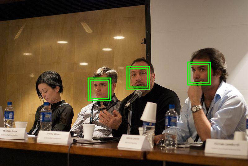
Start with the distinction that trips up almost everyone. Face detection answers "is there a face here, and where?" It draws a box. It is the humble cousin of face recognition, which answers the much harder "whose face is this?" Recognition needs detection first: you cannot match a face to a name until you have isolated the face from the wallpaper behind it. This chapter is entirely about that first step, the boxes, and it turns out the boxes are the part that had to be invented.

Tap the sim's 📷 Camera and move around: lean in, lean out, tilt your head, half-cover your face with a hand. Watch the box lock on, hesitate, and let go. Then 🖼 Upload a group photo and see how many faces it catches at once. Drag the sensitivity slider and notice the trade you are making: crank it up and ghost-faces appear in the noise; crank it down and real faces go missing.

What you just felt in that slider is the central tension of all detection: every detector lives on a line between false positives (calling a cloud a face) and false negatives (missing a real one). You cannot have zero of both. The whole craft is choosing where on that line to sit, and building a detector fast enough to test that choice millions of times across an image before the next video frame arrives.

The atom of the classic detector is a single number computed from a rectangle of the image: the brightness on one side minus the brightness on the other.

$$f = \sum_{(x,y) \in \text{white}} I(x,y) \; - \; \sum_{(x,y) \in \text{black}} I(x,y)$$

Here $f$ is the feature value, a single scalar verdict for one little template laid over one spot in the image. $I(x,y)$ is the intensity (brightness) of the pixel at column $x$, row $y$. The two sums add up all the pixel brightnesses under the "white" half of the template and under the "black" half, and we subtract. If $f$ is large, the dark region really is darker than the light region: evidence that the structure the template is hunting for is present.

The features that look like nothing and mean everything

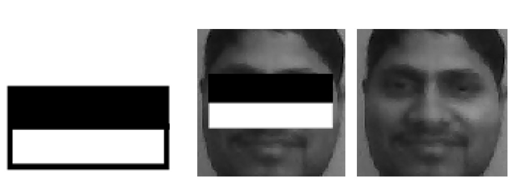
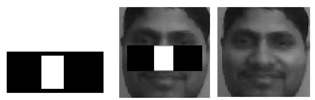
The templates are called Haar-like features, and they could not be simpler: rectangles of paired light and dark zones. An edge feature is two side-by-side bars. A line feature is a dark bar flanked by light ones. A four-rectangle feature is a checkerboard.

They are named for their resemblance to the Haar wavelets, the staircase functions Hungarian mathematician Alfréd Haar published in 1909, long before any image was digital. The link to vision came in stages: a 1998 paper by Constantine Papageorgiou, Michael Oren, and Tomaso Poggio proposed describing objects with a Haar-wavelet feature set instead of raw pixel intensities, because working directly with RGB values made every calculation ruinously expensive. Paul Viola and Michael Jones adapted that idea into the specific rectangle templates we now call Haar-like.

Why would such crude templates detect something as intricate as a face? Because a face, viewed as a topography of light and dark, is astonishingly consistent. The eye sockets are darker than the cheeks below them. The bridge of the nose catches light and is brighter than the eyes on either side. These relationships hold across skin tones, across people, across most lighting, because they come from the geometry of the skull and the way it shades itself, not from any one person's appearance.

The trick that made it real-time: the integral image

A single Haar feature is cheap. The problem is that there are hundreds of thousands of them (every template, at every size, at every position) and you must evaluate them across an image scanned at many scales. Summing thousands of pixels per feature, per location, per scale, is hopeless at video rates.

The escape is a precomputed table called the integral image (or summed-area table). At each pixel it stores the sum of all pixels above and to the left of it:

$$\text{II}(x,y) = \sum_{x' \le x,\; y' \le y} I(x', y')$$

$\text{II}(x,y)$ is the running total of brightness in the entire rectangle from the top-left corner down to $(x,y)$. You build this whole table in one pass over the image. The payoff is that the sum of pixels inside any rectangle, no matter how large, is then four table lookups and three additions:

$$\sum_{\text{rect}} I = \text{II}(D) - \text{II}(B) - \text{II}(C) + \text{II}(A)$$

where $A, B, C, D$ are the rectangle's four corners. Constant time, regardless of rectangle size. Viola and Jones reported that a two-rectangle feature costs roughly sixty processor instructions. That single data structure is what turned "in principle possible" into "fifteen frames a second on a 700 MHz Pentium III in 2001."

AdaBoost and the cascade: a committee that quits early

A single Haar feature is a weak learner: barely better than a coin flip at telling face from not-face. The genius is in how you combine thousands of them. Viola and Jones used AdaBoost (adaptive boosting, the algorithm Yoav Freund and Robert Schapire introduced in 1995) to do two jobs at once: pick, out of the 180,000-odd candidate features, the small handful that matter most, and weight each chosen feature by how much to trust it. A boosted committee of even a few hundred weak rectangles becomes a strong classifier.

But running the full committee on every window is still too slow, because the overwhelming majority of windows in any photo are obviously not faces (sky, wall, sleeve) and deserve none of that effort. So the features are arranged into a cascade: a sequence of stages, ordered from cheap to expensive.

• Stage 1 uses a couple of features and rejects roughly half of all non-face windows instantly.
• Each later stage uses more features and demands a higher standard.
• A window that fails any stage is thrown out immediately and never seen again.
• Only a window that survives every stage is declared a face.

This is the asymmetry that wins: faces are rare, so almost every window is rejected in the first stage or two, costing almost nothing. The expensive deep checks only ever run on the few candidates that already look promising. It is a bouncer at the door rejecting the obvious before the detailed interview ever happens.

The full detection loop then reads as: scan the image with a sliding window at many scales; at each window run the cascade; if every stage passes, mark a face; finally apply non-maximum suppression to collapse the cluster of overlapping boxes a real face triggers into a single tidy rectangle. The sensitivity slider in the sim is, in spirit, the threshold those stages compare against.

↘ For the advanced reader → How AdaBoost builds a strong classifier from rectangles that are barely better than chance

AdaBoost builds a strong classifier $H(x)$ as a weighted vote of $T$ weak classifiers $h_t(x)$, each of which is a single Haar feature thresholded into a yes/no:

$$H(x) = \operatorname{sign}\!\left( \sum_{t=1}^{T} \alpha_t \, h_t(x) \right)$$

Training is iterative. Every training image $i$ carries a weight $w_i$, initially uniform. On round $t$ the algorithm picks the single feature whose thresholded classifier $h_t$ has the lowest weighted error $\varepsilon_t$ on the current weights. The trust given to that classifier is

$$\alpha_t = \tfrac{1}{2}\ln\!\left( \frac{1 - \varepsilon_t}{\varepsilon_t} \right)$$

so a near-perfect feature ($\varepsilon_t \to 0$) earns a large $\alpha_t$, while one near chance ($\varepsilon_t \to 0.5$) earns almost none. Then the weights are updated to emphasize the examples this round got wrong:

$$w_i \leftarrow w_i \, \exp\!\big(\!-\alpha_t \, y_i \, h_t(x_i)\big), \qquad y_i \in \{-1, +1\}$$

followed by renormalizing so the weights sum to one. Misclassified examples grow heavier, so the next round is forced to attend to the cases the committee still fails. Each weak learner patches the previous committee's blind spots.

The cascade layers a second optimization on top. If each stage $k$ achieves detection rate $d_k$ and false-positive rate $f_k$, then a cascade of $K$ stages has overall rates

$$D = \prod_{k=1}^{K} d_k, \qquad F = \prod_{k=1}^{K} f_k.$$

Because the $f_k$ multiply, even modest per-stage false-positive rates (say $0.5$) drive $F$ toward zero exponentially: ten stages at $0.5$ each give $F \approx 0.001$. Meanwhile each $d_k$ is kept very close to $1$ (say $0.997$) so their product $D$ stays high. The design problem is choosing the number of stages and per-stage thresholds to hit a target $(D, F)$ at the least average computation, knowing nearly every window dies in the first one or two stages.

After Viola-Jones: when faces stopped lying flat

The classic cascade has a real weakness: it loves frontal, upright faces and struggles with profiles, big tilts, and heavy occlusion, because its rectangle features assume the eyes-nose-cheeks geometry it was trained on. The deep-learning era answered this. MTCNN runs a multi-task cascade of small neural networks that find the face and its key landmarks together. RetinaFace pushed accuracy to the state of the art with dense landmark and 3D supervision. And BlazeFace, the model running in the sim above, is engineered for phones: a lightweight network that returns face boxes in well under a millisecond on a mobile GPU.

Key takeaways

• Detection is not recognition. Face detection draws the box ("a face is here"); face recognition reads the name. Recognition always runs after detection, on the cropped result.
• Haar-like features are sums of light and dark rectangles, crude templates that work because the face's topography (dark eyes, bright nose bridge, lit forehead) is consistent across people and lighting.
• The integral image makes any rectangle sum a constant-time, four-lookup operation, which is the single trick that turned face detection into a real-time, real-world capability in 2001.
• AdaBoost selects and weights the few features that matter, and the cascade rejects obvious non-faces in its first cheap stages, spending real effort only on the rare promising windows.
• Deep models (MTCNN, RetinaFace, BlazeFace) now lead on accuracy and pose, but the compact Viola-Jones cascade endures wherever power, memory, and cost are scarce.