Contour Detection
Finding Shapes
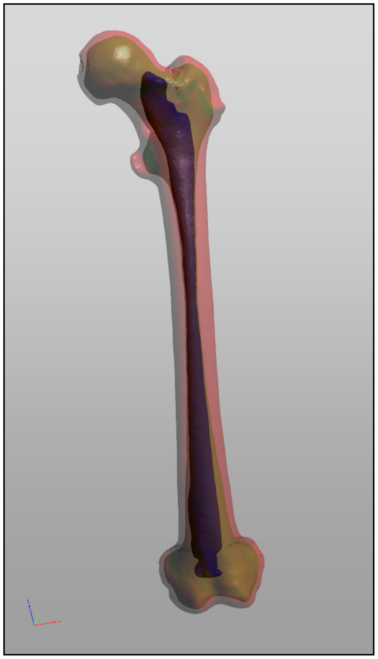
A radiologist scrolls through a stack of CT slices. On each one, a pale ring of bone floats against darker tissue. Her eye, without effort, closes that ring into a single thing: femur. Slice after slice, the rings stack, and a leg bone takes shape in her mind in three dimensions.
A computer cannot see the femur. It sees a grid of numbers. To make it perceive the bone, you have to teach it to do what her eye did instantly: walk along the edge of the bright region, never lifting the pen, and come back to where it started. That traced loop is a contour, and once you have it you can measure the bone, count the bones, match this bone against a library of bones.
A contour is the act of closing an edge into a shape: the moment a boundary stops being a scatter of pixels and becomes an object you can hold.
The previous chapters gave us edges: places where brightness changes sharply. But an edge is a local verdict, a yes-or-no at a single pixel. It does not know whether it belongs to the same coin as the edge two pixels over. Contour detection is the step that stitches those local edges into a complete, ordered, closed boundary, so that "the outline of the coin" becomes one connected list of points you can reason about as a whole.
Trace it yourself
The simulator below takes an image, thresholds it into pure black-and-white, then walks the borders of every white region and draws each traced loop in its own color. Drag the threshold slider and watch the outlines snap to the shapes. Then tap Camera and point it at something with strong contrast (a dark pen on white paper works beautifully). Look for the moment when a single blob splits into two as the threshold crosses a critical value: that is the algorithm rediscovering the boundary in real time.
What you just watched is the whole pipeline in miniature. The threshold turns a continuous image into a binary mask of "object" and "not object." The tracer then follows the staircase frontier between the two, recording each turn as a point, until it returns home. Notice that the result is fundamentally different from an edge map: an edge map is a fog of bright pixels, while a contour is an ordered sequence with a beginning, an end (which equals the beginning), and an inside.
From threshold to closed loop
The governing idea is simple to state. A binary image assigns every pixel a label,
where is the original intensity at column , row , and is the threshold you chose. A pixel is a boundary pixel when it is foreground () but has at least one background neighbor (). A contour is then the ordered set of boundary pixels you reach by always keeping the foreground on the same side as you walk:
Here each is a boundary pixel, and the closure condition says the walk ends where it began. That last line is the whole difference between an edge and a contour: the loop closes.
The Suzuki-Abe tracer
OpenCV's findContours implements an algorithm published in 1985 by Satoshi Suzuki and Keiichi Abe, "Topological structural analysis of digitized binary images by border following." Its insight is that you can trace every boundary in a single raster scan, top to bottom, left to right. When the scan hits a transition from background to foreground, it has found a new border. It then "follows" that border all the way around, marking each pixel with a unique border number, before resuming the scan. Because each border gets its own label, the algorithm recovers not just the shapes but how they nest.
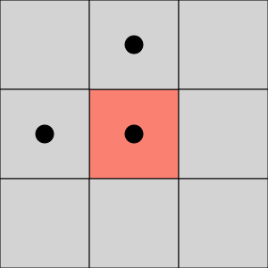
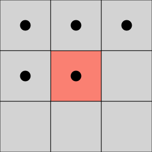
The choice between 4-connectivity and 8-connectivity is not academic. It decides whether two regions touching only at a corner count as one object or two, and it is a perennial source of off-by-one bugs in blob counting. The convention that keeps borders self-consistent is to treat foreground and background with opposite connectivities: if foreground pixels connect 8-ways, background connects 4-ways, and vice versa.
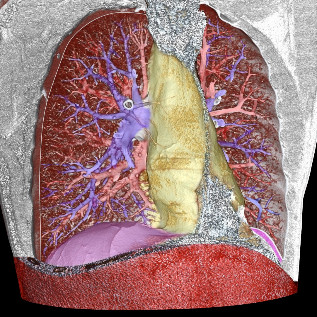
Hierarchy: shapes inside shapes
Contours are rarely lonely. A letter "O" has an outer ring and an inner ring; a washer has a disk and a hole; a face has eyes inside a head. Suzuki and Abe's real contribution was tracking this nesting as a hierarchy: every contour records its parent, its first child, and its siblings.
- An outer (external) contour is the boundary between an object and the background that surrounds it.
- A hole (internal) contour is the boundary between an object and a background region trapped inside it.
OpenCV exposes this through retrieval modes. RETR_EXTERNAL keeps only the outermost loops. RETR_TREE reconstructs the full parent-child forest, so you can say with certainty that this hole lives inside that disk. The hierarchy is stored as four indices per contour: next sibling, previous sibling, first child, and parent, with marking "none."
What a contour tells you
Once a boundary is a closed point list, it stops being a picture and becomes geometry you can measure. The key descriptors:
- Area : how much region the loop encloses, computed with the shoelace formula, not by counting pixels.
- Perimeter : the total length of the boundary, the sum of segment lengths around the loop.
- Centroid : the center of mass of the enclosed region, found from image moments.
- Bounding box: the smallest axis-aligned rectangle that contains the loop.
- Convex hull: the rubber-band polygon you get by stretching an elastic around the shape.
The area and centroid both fall out of image moments. The raw moment of order for a region is
so is simply the pixel count (the area), and the centroid is the first moments normalized by the zeroth:
Each symbol earns its keep: totals the region, weights every pixel by its column, weights by its row, and dividing cancels the size so only the position survives.
For the advanced reader → How seven numbers recognize a shape regardless of how it is moved, sized, or spun
To match shapes you want descriptors that ignore where the shape sits, how big it is, and which way it points. The path runs in three steps.
First, recenter. The central moments subtract the centroid so the descriptor no longer cares about position:
Second, rescale. Dividing by a power of the area removes the dependence on size, giving the normalized central moments:
Third, combine them so rotation cancels too. In 1962 Ming-Kuei Hu showed that seven specific polynomial combinations of the are invariant to translation, scale, and rotation. The first two are
These Hu moments are why OpenCV's matchShapes can decide that a logo photographed from across a room, tilted and shrunk, is the same logo it has in its catalog. Two shapes with nearly equal Hu vectors are geometrically the same shape, full stop.
A related simplification is the Douglas-Peucker algorithm, which thins a contour of hundreds of points down to a handful of corners by recursively discarding points that lie close to the line between their neighbors. Run it on a quadrilateral and you get back exactly four vertices: the basis of every "this contour has 4 sides, it might be a document" detector.
Key takeaways
- A contour closes an edge into an object. Edges are an unordered raster of bright pixels; a contour is an ordered, closed point list that bounds a region you can measure.
- Threshold, then trace. The standard pipeline binarizes the image, then follows the staircase frontier between foreground and background until the walk returns to its start.
- The Suzuki-Abe algorithm (1985) traces every border in one scan and, crucially, records how contours nest, giving you the parent-child hierarchy that distinguishes a hole from an outline.
- Connectivity is a real choice. 4- versus 8-connectivity decides whether corner-touching blobs are one object or two; mismatched connectivity is a classic counting bug.
- Moments turn shape into numbers. Area, centroid, and the rotation/scale/translation-invariant Hu moments let you count, locate, and match shapes, the backbone of OCR, gesture recognition, and 3D reconstruction.
The radiologist's eye closed each pale ring into a bone without her ever naming the act. We have now named it, and broken it into steps a machine can follow: set a threshold, keep the foreground on your left, walk until you come home. Do that on every slice and the loops stack into a femur; do it on a page and the loops resolve into letters; do it on a hand and the loops count the fingers.
A contour is the smallest unit of seeing a thing as a thing. Everything downstream, every measurement, every match, every reconstruction, begins the instant the pen returns to where it started.