Pixels & Color Spaces
The Digital Image
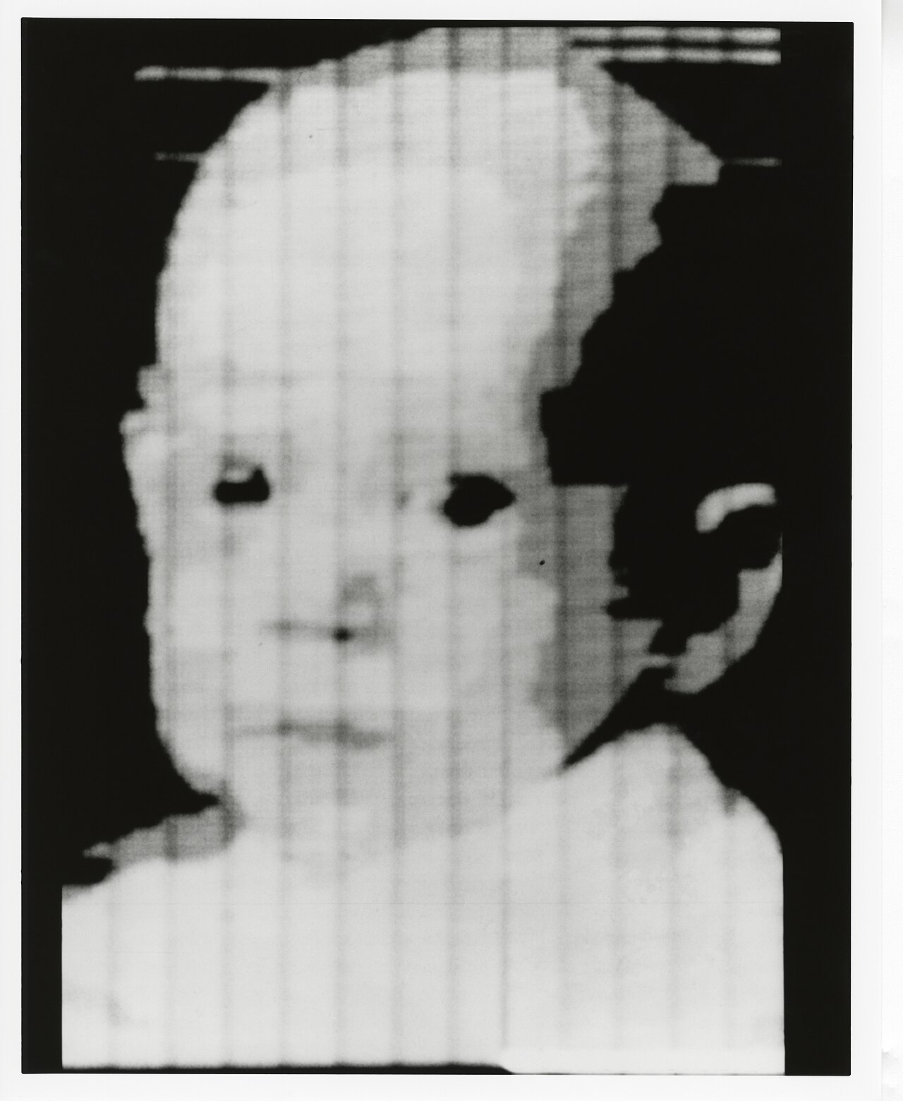
In 1957, a researcher at the U.S. National Bureau of Standards laid a small black-and-white photo of his three-month-old son on a rotating drum scanner and asked a question nobody had asked before: what if a picture were just a list of numbers?
The machine, a room-sized computer called SEAC, sampled the photo into a grid 176 squares wide and 176 squares tall. Each square got one number for how bright it was. The result was a smudged, blocky little face, the size of a postage stamp. It was also the first digital image in history.
Every image a computer has ever seen, from your phone's selfie to a Mars rover's panorama, is the same idea: light, chopped into a grid of numbers.
Before a computer can find a face, track a ball, or measure a star, it has to do something stranger and more humble first: it has to turn a continuous flood of light into something it can count. That something is a grid of tiny samples called pixels, short for "picture element." Each pixel is one little bucket that holds a number (or a few numbers) describing the color of light that landed there. Vision, for a machine, begins as arithmetic on that grid.
This lesson is about those numbers: how many you need per pixel, what each one means, and the surprising fact that the same color can be written down in many different ways. Those different ways of writing color are called color spaces, and choosing the right one is often the difference between an algorithm that works and one that falls apart the moment a cloud passes over the sun.
Try it: one color, three coordinate systems
Drag the color picker below through RGB (the red-green-blue sliders), then watch the HSV readout change in lockstep. Pick a vivid red, then slowly drag it darker: notice how the Hue number stays put while Value drops. Then tap 📷 Camera to let the sim decompose your real room, pixel by pixel, into channels.
What you just watched is the central trick of this whole chapter. A single color is one physical thing, but you can address it with different sets of coordinates. RGB describes it by how much of each light to mix. HSV describes it by what color it is, how pure, and how bright. Neither is more "correct." They are two maps of the same territory, and computer vision constantly translates between them because each map makes different problems easy.
A pixel is a sample, and a sample is a number
The minimal definition is small enough to hold in one hand. A grayscale pixel is a single integer, almost always in the range to :
Here is the image, a function you can query. The inputs and are the column and row of the pixel (its address in the grid). The output is the intensity: means no light reaching that spot (black), means fully saturated light (white), and everything between is a shade of gray. The range stops at because the value is stored in 8 bits, and . That single byte per pixel is the atom of digital imaging.
Stack many of these samples in a grid and you have the image as a matrix: rows by columns. A modest 1920×1080 photo holds pixels. In full color, with three bytes each, that is over six megabytes of raw numbers for a single frame, before any compression.
When pixels are big enough to see with the naked eye, you get pixel art: the chunky, deliberate aesthetic of early video games, born not from style but from the brutal memory limits of 1980s hardware. The blockiness was a constraint that later became a language.
RGB: building color by adding light
Look at that macro photo again. Your screen has no "yellow" lamp and no "pink" lamp. It only has red, green, and blue emitters, packed so densely that your eye blends them. This is the RGB color model, and it is additive: you start from darkness and add colored light to climb toward white. Red plus green light makes yellow. All three at full blast make white. All three off is black.
This is the opposite of how paint works. Mixing red, green, and blue paint gives a muddy brown, because pigments subtract light, absorbing wavelengths rather than emitting them. Printers live in that subtractive world and use a different set of primaries, cyan-magenta-yellow-black (CMYK). The deep reason your monitor and your printer disagree about color is that one adds light and the other takes it away.

A subtle but important fact: RGB is device-dependent. The exact red your phone emits is not the exact red your laptop emits, because the physical emitters differ between manufacturers and even drift as a screen ages. An RGB triple like is therefore an instruction ("turn the red emitter all the way up"), not an absolute description of a color. Pinning RGB numbers to physically real, repeatable colors requires a reference standard, which is the whole reason color spaces like sRGB and Adobe RGB exist.
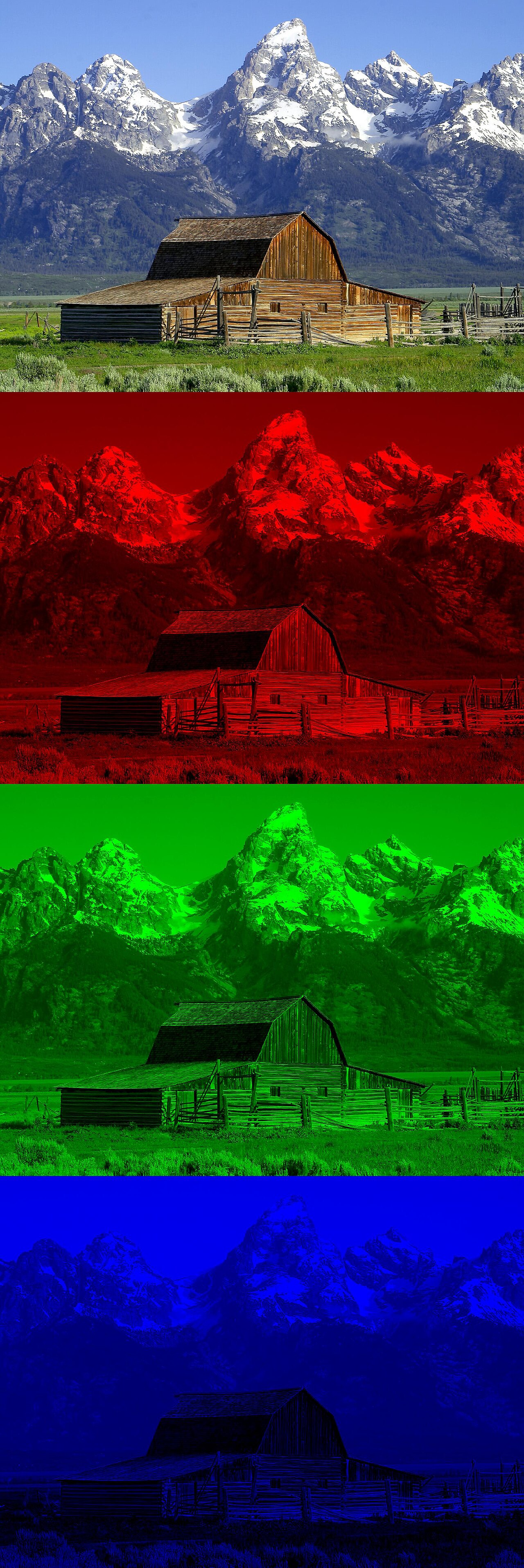
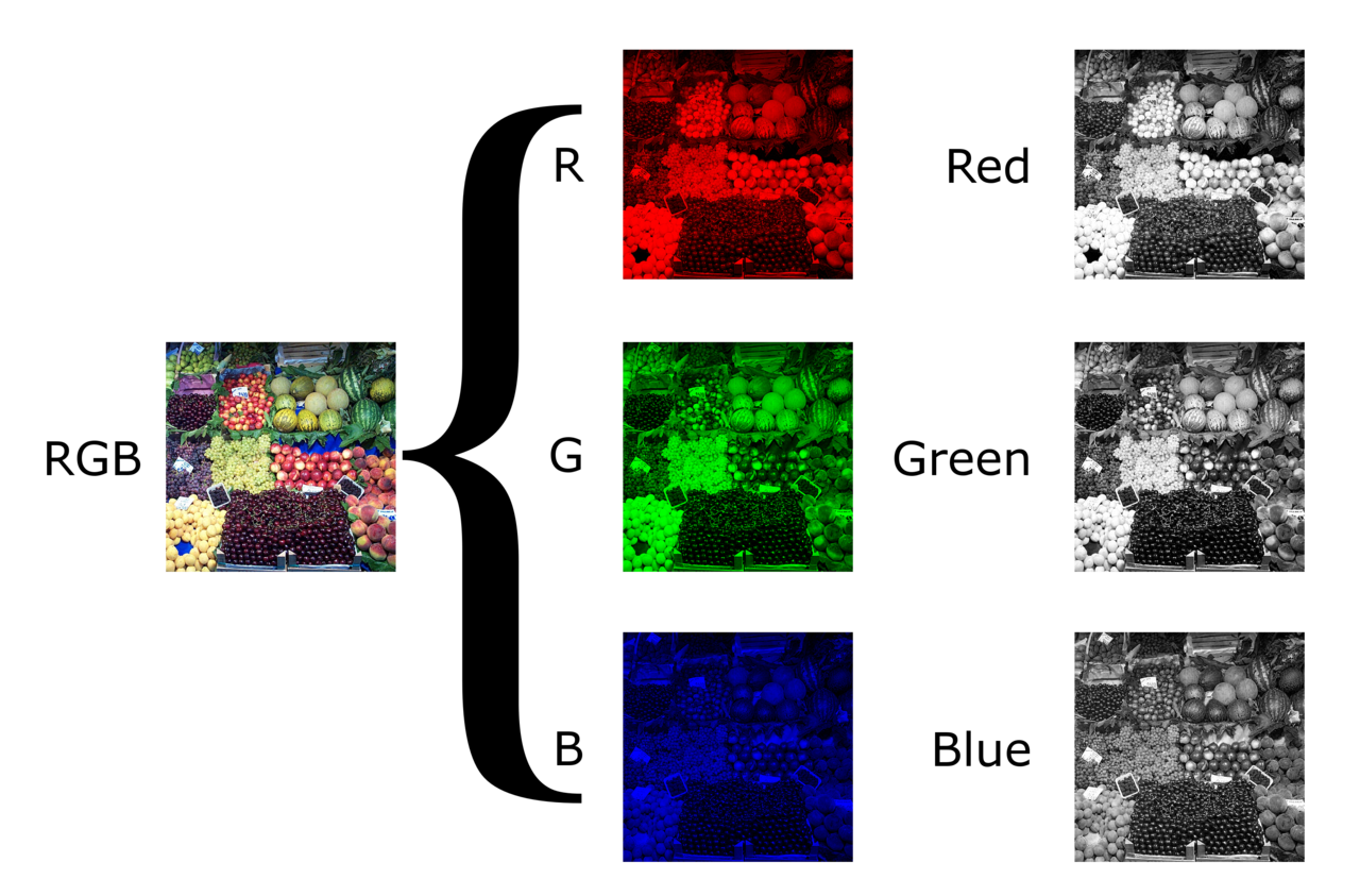
You can split any photo into its three channels and view each one as a grayscale image. Bright areas in the "red" channel are the parts of the scene that reflected a lot of red light. This decomposition is the raw material almost every vision pipeline starts from.
Grayscale: throwing away color on purpose
A great deal of computer vision begins by deleting color entirely. Edge detection, corner finding, and many feature detectors only care about brightness, so collapsing three channels into one makes them three times cheaper and often more robust. The naive way to do this would be to average the channels equally, but that produces grays that look wrong to human eyes.
The standard conversion weights the channels unequally:
Each symbol here is the intensity of one channel for a single pixel: , , and are red, green, and blue (each to ), and is the resulting gray, called luma. The weights are not arbitrary. They mirror the sensitivity of human vision: our eyes have far more receptors tuned to green, so green contributes more than half the perceived brightness, while blue, which we see most poorly, contributes barely a tenth. A pure-green and a pure-blue light of equal physical energy look wildly different in brightness to us, and these weights bake that fact in.
HSV: the color space that survives a passing cloud
RGB is how screens make color, but it is a clumsy way to reason about color. Suppose you want a robot to track a red ball. In RGB, "red" is a fuzzy, sprawling region: the ball in shadow might be and in sunlight , and there is no single, simple rule that captures both. The brightness change has scrambled all three numbers at once.
In the 1970s, computer-graphics researchers rearranged the RGB cube into a cylinder to fix exactly this. The result, HSV (Hue, Saturation, Value), gives color three more intuitive coordinates:
- Hue is the angle around the cylinder ( to ): the pure color, red at , green near , blue near . This is what color it is.
- Saturation is the distance from the central axis ( to ): how vivid versus washed-out the color is. This is how pure it is.
- Value is the height along the axis ( to ): how bright or dark. This is how much light there is.
The payoff is that brightness lives in a single coordinate. When that cloud passes over the sun, mostly only Value drops; the Hue of the red ball barely moves. So "track the red ball" becomes a simple, stable rule: keep every pixel whose Hue is near red, regardless of Value. That single property is why HSV (and its cousins HSL and HSI) shows up in nearly every color-tracking system ever built.
For all its convenience, HSV is a crude approximation of human perception. It is a quick mathematical reshuffle of device-dependent RGB, not a model grounded in how the eye actually works. When perceptual accuracy truly matters (matching paint colors, grading film), engineers reach for heavier, perceptually-uniform spaces like CIELAB, which were designed from measurements of human color vision rather than from the geometry of a screen.
The exact RGB-to-HSV conversion, derived from the cube's geometry
Normalize each channel to the range by dividing by , then let
is the brightest channel, the dimmest, and is the chroma: how far the color is from gray. Value is simply the brightest channel:
Saturation is chroma measured relative to that brightness (zero when the color is gray, since then ):
Hue is the angular position, computed piecewise depending on which channel is the maximum:
The factor converts the six segments of the hexagonal cross-section into a full wheel. Notice that Hue is undefined when : a perfectly gray pixel has no color direction, the same way the North Pole has no longitude. This is the source of countless flickering artifacts in naive color-tracking code that forgets to guard the achromatic case.
Key takeaways
- A pixel is just a sample of light, stored as a number. Grayscale uses one byte per pixel (–); color uses three or four. An image is a matrix of these numbers indexed by row and column.
- RGB is additive and device-dependent. It mixes red, green, and blue light to climb from black to white, and the same triple can look different on different screens, which is why color spaces (sRGB, Adobe RGB) exist to anchor it.
- Grayscale conversion is weighted, not averaged. The formula encodes the eye's strong green sensitivity and weak blue sensitivity.
- HSV separates color from brightness. Putting Hue, Saturation, and Value on independent axes makes color-based detection robust to changing light, the single most useful property in practical color tracking.
- The right color space makes a hard problem easy. Choosing among RGB, grayscale, HSV, and YCbCr is a real engineering decision, not a formality.
Russell Kirsch's blurry little portrait of his son was pixels wide because that was all the memory the machine could spare. Today your pocket holds cameras that gulp tens of millions of pixels at a time, in full color, sixty times a second.
But the bargain has never changed. To see, a computer must first agree to forget: to throw away the smooth continuity of the world and accept a grid of numbers in its place. Everything that follows in this book (every edge, every face, every reconstructed 3D scene) is built on that grid, and on the quiet decision of how, exactly, to write down the color of light.